A program that works for either single or double precision

Now let's look at a function to compute enough terms in the Fibonacci sequence so the ratio is less than the correct machine epsilon (eps) for datatype single or double. % How many terms needed to get single precision results?

fibodemo('single')

% How many terms needed to get double precision results?

fibodemo('double')

% Now let's look at the working code.

type fibodemo

% Notice that we initialize several of our variables, |fcurrent|,

% |fnext|, and |goldenMean|, with values that are dependent on the

% input datatype, and the tolerance |tol| depends on that type as

% well. Single precision requires that we calculate fewer terms than

% the equivalent double precision calculation.

ans = 19

ans = 41

function nterms = fibodemo(dtype)

%FIBODEMO Used by SINGLEMATH demo.

% Calculate number of terms in Fibonacci sequence.

fcurrent = ones(dtype);

fnext = fcurrent;

goldenMean = (ones(dtype)+sqrt(5))/2;

tol = eps(goldenMean);

nterms = 2;

while abs(fnext/fcurrent - goldenMean) >= tol

nterms = nterms + 1;

temp = fnext;

fnext = fnext + fcurrent;

fcurrent = temp;

end

Inverses of Matrices

This demo shows how to visualize matrices as images and uses this to illustrate matrix inversion.

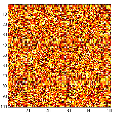
This is a graphic representation of a random matrix. The RAND command creates the matrix, and the IMAGESC command plots an image of the matrix, automatically scaling the color map appropriately.

n = 100;

a = rand(n);

imagesc(a);

colormap(hot);

axis square;

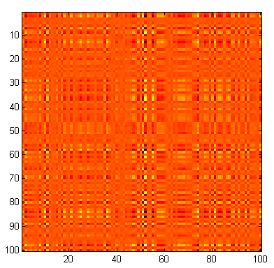
This is a representation of the inverse of that matrix. While the numbers in the previous matrix were completely random, the elements in this matrix are anything BUT random. In fact, each element in this matrix ("b") depends on every one of the ten thousand elements in the previous matrix ("a").

b = inv(a);

imagesc(b);

axis square;

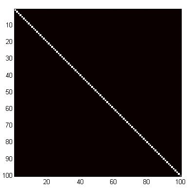
But how do we know for sure if this is really the correct inverse for the original matrix? Multiply the two together and see if the result is correct, because just as 3*(1/3) = 1, so must a*inv(a) = I, the identity matrix. The identity matrix (almost always designated by I) is like an enormous number one. It is completely made up of zeros, except for ones running along the main diagonal.

This is the product of the matrix with its inverse: sure enough, it has the distinctive look of the identity matrix, with a band of ones streaming down the main diagonal, surrounded by a sea of zeros.

imagesc(a*b);

axis square;

Graphs and Matrices

This demo gives an explanation of the relationship between graphs and matrices and a good application of SPARSE matrices.

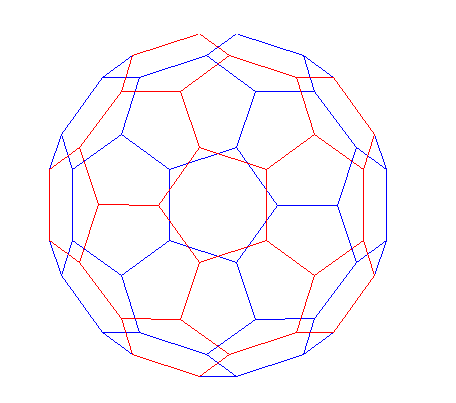
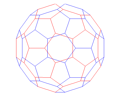
A graph is a set of nodes with specified connections between them. An example is the connectivity graph of the Buckminster Fuller geodesic dome (also a soccer ball or a carbon-60 molecule).

In MATLAB, the graph of the geodesic dome can be generated with the BUCKY function.% Define the variables.

[B,V] = bucky;

H = sparse(60,60);

k = 31:60;

H(k,k) = B(k,k);

% Visualize the variables.

gplot(B-H,V,'b-');

hold on

gplot(H,V,'r-');

hold off

axis off equal

A graph can be represented by its adjacency matrix.

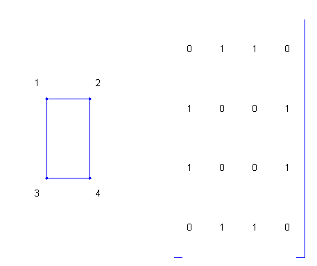
To construct the adjacency matrix, the nodes are numbered 1 to N. Then element (i,j) of the matrix is set to 1 if node i is connected to node j, and 0 otherwise. % Define a matrix A.

A = [0 1 1 0 ; 1 0 0 1 ; 1 0 0 1 ; 0 1 1 0];

% Draw a picture showing the connected nodes.

cla

subplot(1,2,1);

gplot(A,[0 1;1 1;0 0;1 0],'.-');

text([-0.2, 1.2 -0.2, 1.2],[1.2, 1.2, -.2, -.2],('1234')', ...

'HorizontalAlignment','center')

axis([-1 2 -1 2],'off')

% Draw a picture showing the adjacency matrix.

subplot(1,2,2);

xtemp=repmat(1:4,1,4);

ytemp=reshape(repmat(1:4,4,1),16,1)';

text(xtemp-.5,ytemp-.5,char('0'+A(:)),'HorizontalAlignment','center');

line([.25 0 0 .25 NaN 3.75 4 4 3.75],[0 0 4 4 NaN 0 0 4 4])

axis off tight

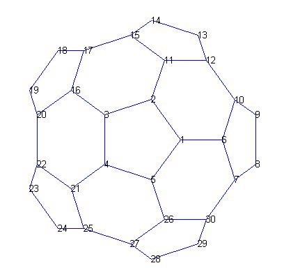
Here are the nodes in one hemisphere of the bucky ball, numbered polygon by polygon.subplot(1,1,1);

gplot(B(1:30,1:30),V(1:30,:),'b-')

for j = 1:30,

text(V(j,1),V(j,2),int2str(j),'FontSize',10);

end

axis off equal

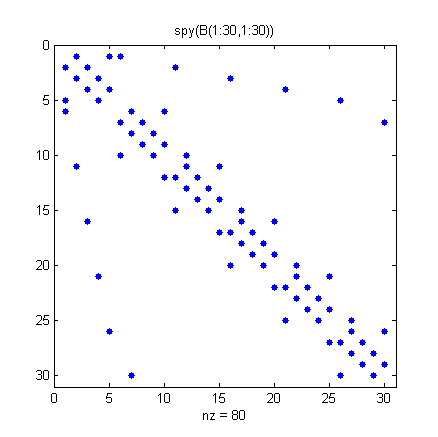
To visualize the adjacency matrix of this hemisphere, we use the SPY function to plot the silhouette of the nonzero elements.

Note that the matrix is symmetric, since if node i is connected to node j, then node j is connected to node i.

spy(B(1:30,1:30))

title('spy(B(1:30,1:30))')

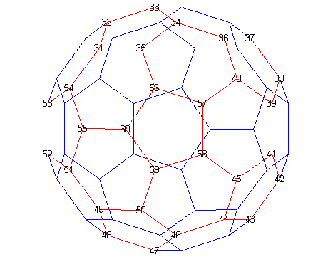
numbering of one hemisphere into the other.

[B,V] = bucky;

H = sparse(60,60);

k = 31:60;

H(k,k) = B(k,k);

gplot(B-H,V,'b-');

hold on

gplot(H,V,'r-');

for j = 31:60

text(V(j,1),V(j,2),int2str(j), ...

'FontSize',10,'HorizontalAlignment','center');

end

hold off

axis off equal

Finally, here is a SPY plot of the final sparse matrix.

spy(B)

title('spy(B)')

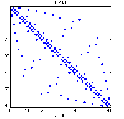
In many useful graphs, each node is connected to only a few other nodes. As a result, the adjacency matrices contain just a few nonzero entries per row.

This demo has shown one place where SPARSE matrices come in handy.gplot(B-H,V,'b-');

axis off equal

hold on

gplot(H,V,'r-')

hold off